Liquidations are one of the most important events in crypto derivatives markets. When leveraged positions get forcibly closed, they create selling (or buying) pressure that can cascade into dramatic price moves. Understanding liquidation data gives you insight into market stress and potential reversal points.
In this tutorial, we'll analyze real liquidation data from Binance Futures to:
- Find the biggest liquidation events (top 10 long and short windows)
- Measure price impact during and after major liquidations
- Compare liquidation patterns during different market conditions
What Are Liquidations?
When a trader opens a leveraged position on a futures exchange, they must maintain a minimum margin. If the position moves against them and their margin drops below the maintenance requirement, the exchange forcibly closes their position—this is a liquidation.
- Long liquidation: A long position is force-closed by selling. This creates downward price pressure.
- Short liquidation: A short position is force-closed by buying. This creates upward price pressure.
Liquidations tend to cluster because they're self-reinforcing: a price drop causes long liquidations, which creates more selling pressure, which causes more long liquidations. Finding these clusters reveals the most significant market stress events.
Loading Liquidation Data
Let's start by loading liquidation data from CryptoHFTData:
import cryptohftdata as chd
import pandas as pd

# Configure API
chd.configure_client(api_key="your-api-key-here")

# Load liquidation data (2 weeks)
liqs_df = chd.get_liquidations(
    symbol="BTCUSDT",
    exchange="binance_futures",
    start_date="2025-08-01",
    end_date="2025-08-14"
)

# Preprocess
liqs_df["datetime"] = pd.to_datetime(liqs_df["event_time"], unit="ms")
liqs_df["price"] = pd.to_numeric(liqs_df["average_price"], errors="coerce")
liqs_df["quantity"] = pd.to_numeric(liqs_df["filled_quantity"], errors="coerce")
liqs_df["volume_usd"] = liqs_df["quantity"] * liqs_df["price"]

# Classify liquidation type (SELL = long position liquidated, BUY = short position liquidated)
liqs_df["liq_type"] = liqs_df["side"].apply(
    lambda x: "long" if x == "SELL" else "short"
)
The data includes the execution price, quantity, timestamp, and which side was liquidated.
Data Overview
Over two weeks (August 1-14, 2025), BTCUSDT on Binance Futures saw:
| Metric | Value |
|---|---|
| Total liquidations | 15,108 |
| Total volume | $162.3M |
| Long liquidations (longs rekt) | $78.7M (48.5%) |
| Short liquidations (shorts rekt) | $83.6M (51.5%) |
The liquidation volume was nearly balanced between longs and shorts over the two-week period—quite different from looking at a single day where one side often dominates.
Finding the Top Liquidation Windows
Instead of using statistical thresholds, we take a simpler approach: aggregate liquidations into 5-minute windows and find the top 10 windows for each side. This directly identifies the biggest liquidation events.
def aggregate_by_window(liqs_df, window="5min"):
    """Aggregate liquidations into time windows."""
    df = liqs_df.copy().set_index("datetime")

    # Total aggregation
    agg = df.resample(window).agg({
        "volume_usd": "sum",
        "quantity": "sum",
        "price": "mean",
        "side": "count"
    }).rename(columns={"side": "count", "price": "avg_price"})

    # By side
    long_agg = df[df["liq_type"] == "long"].resample(window)["volume_usd"].sum()
    short_agg = df[df["liq_type"] == "short"].resample(window)["volume_usd"].sum()

    agg["long_volume"] = long_agg.reindex(agg.index, fill_value=0)
    agg["short_volume"] = short_agg.reindex(agg.index, fill_value=0)

    return agg.reset_index()


def find_top_liquidation_windows(agg_df, n=10):
    """Find the top N windows for long and short liquidations."""
    top_long = agg_df.nlargest(n, "long_volume")
    top_short = agg_df.nlargest(n, "short_volume")
    return top_long, top_short
Top 10 Long Liquidation Windows (Longs Getting Rekt)
| Time | Volume | Count | Avg Price |
|---|---|---|---|
| 2025-08-01 13:50 | $3,194,564 | 57 | $114,262 |
| 2025-08-11 18:00 | $2,589,485 | 28 | $119,334 |
| 2025-08-14 12:30 | $2,405,641 | 142 | $119,824 |
| 2025-08-01 00:50 | $2,086,457 | 85 | $114,807 |
| 2025-08-11 11:15 | $2,078,148 | 31 | $120,764 |
| 2025-08-14 06:20 | $1,712,851 | 20 | $121,395 |
| 2025-08-14 06:00 | $1,463,440 | 60 | $121,871 |
| 2025-08-01 19:20 | $1,412,180 | 56 | $113,387 |
| 2025-08-02 18:55 | $1,098,390 | 32 | $112,156 |
| 2025-08-05 12:35 | $941,582 | 54 | $113,924 |
Top 10 Short Liquidation Windows (Shorts Getting Rekt)
| Time | Volume | Count | Avg Price |
|---|---|---|---|
| 2025-08-13 11:10 | $6,638,913 | 6 | $120,671 |
| 2025-08-11 02:50 | $1,971,525 | 12 | $121,813 |
| 2025-08-06 04:05 | $1,142,399 | 9 | $113,404 |
| 2025-08-14 00:20 | $1,084,802 | 12 | $124,013 |
| 2025-08-03 19:35 | $908,324 | 18 | $114,655 |
| 2025-08-11 02:35 | $899,501 | 10 | $121,683 |
| 2025-08-11 09:35 | $885,937 | 6 | $121,171 |
| 2025-08-13 13:50 | $874,808 | 89 | $121,583 |
| 2025-08-04 17:15 | $830,277 | 12 | $115,660 |
| 2025-08-11 03:00 | $823,851 | 8 | $121,923 |
The $6.6M short liquidation window on August 13 was the largest single event—shorts got squeezed hard as BTC pumped through $120k. Notice how short liquidation windows tend to have fewer individual liquidations but larger average sizes.
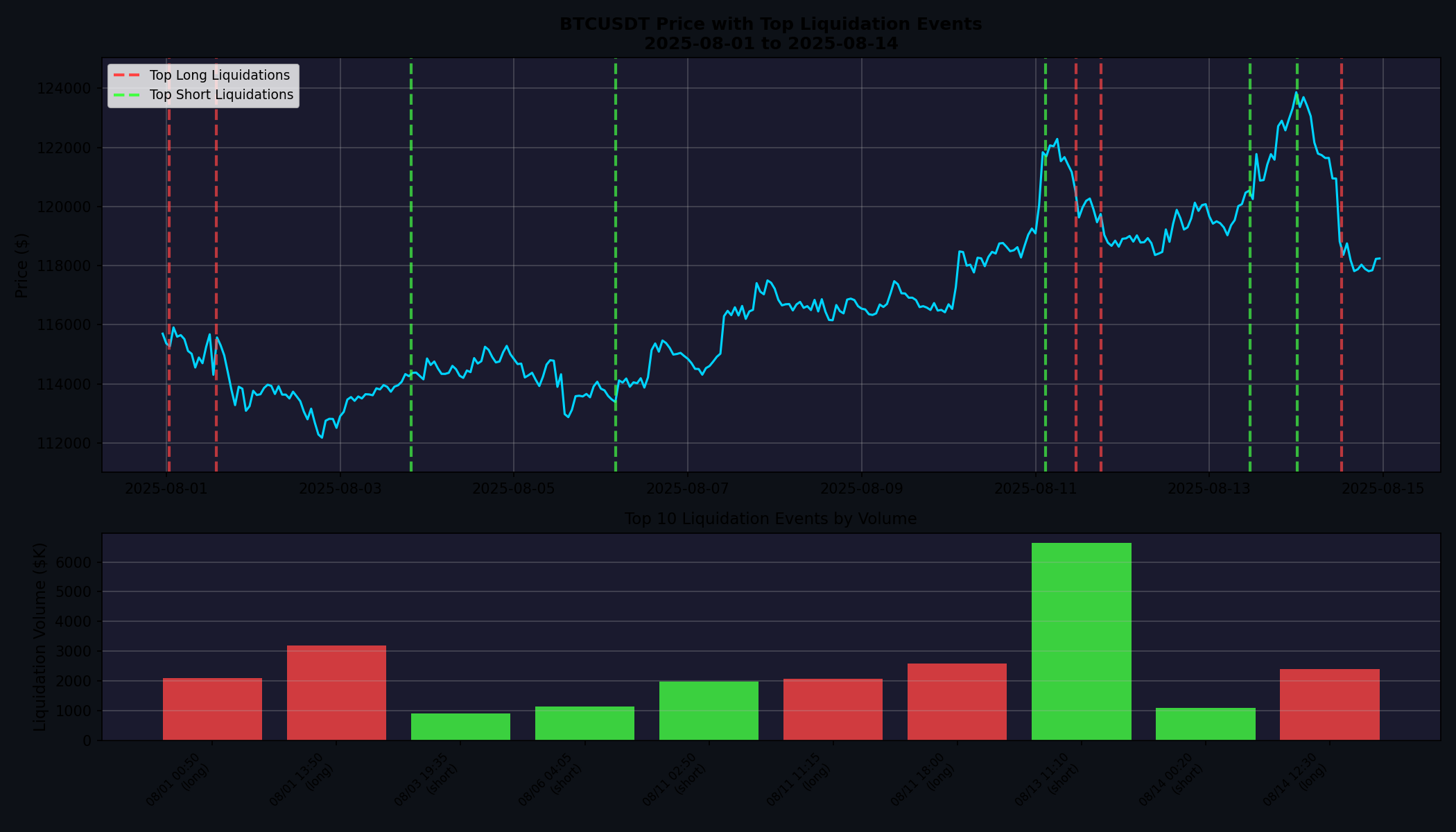
The chart shows price with the top 5 long (red) and short (green) liquidation events marked. You can see how these cluster around sharp price movements.
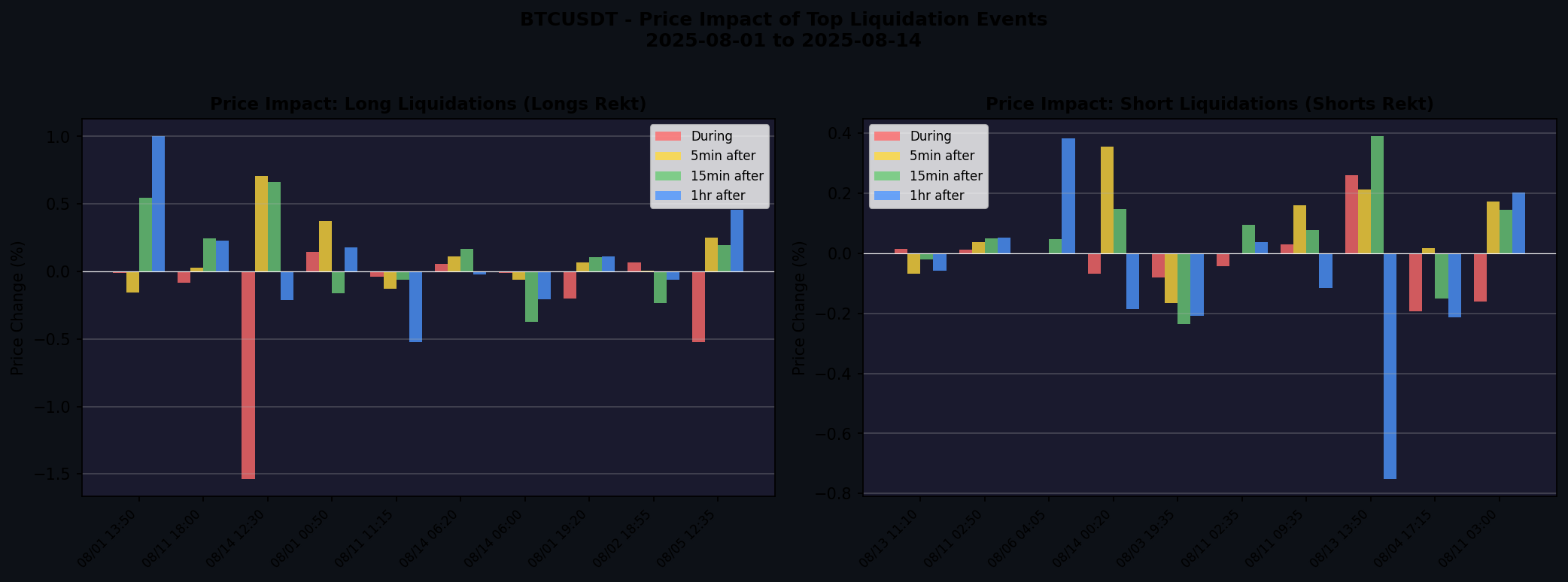
Price Impact Analysis
The key question: what happens to price during and after these major liquidation events? We measure price change during the 5-minute window, then 5 minutes, 15 minutes, and 1 hour after.
def calculate_price_impact(events_df, price_df, window_minutes=5):
    """Calculate price movement during and after each event window."""
    results = []

    for _, event in events_df.iterrows():
        event_time = event["datetime"]
        event_end = event_time + pd.Timedelta(minutes=window_minutes)

        # Price at window start
        pre = price_df[price_df["datetime"] <= event_time]
        price_start = pre.iloc[-1]["close"]

        # Price at window end
        post = price_df[price_df["datetime"] >= event_end]
        price_end = post.iloc[0]["close"]

        # Price at various intervals after
        for minutes, label in [(5, "5min"), (15, "15min"), (60, "1hr")]:
            after = price_df[price_df["datetime"] >= event_end + pd.Timedelta(minutes=minutes)]
            if len(after) > 0:
                change = (after.iloc[0]["close"] - price_end) / price_end * 100
                result[f"change_{label}_after"] = change

        result["change_during"] = (price_end - price_start) / price_start * 100
        results.append(result)

    return pd.DataFrame(results)
Long Liquidations (Longs Rekt) - Price Impact
| Metric | Mean | Median | Min | Max |
|---|---|---|---|---|
| Price change during | -0.21% | -0.03% | -1.54% | +0.15% |
| Price change 5 min after | +0.12% | +0.05% | -0.16% | +0.71% |
| Price change 15 min after | +0.11% | +0.14% | -0.38% | +0.66% |
| Price change 1 hour after | +0.10% | +0.05% | -0.53% | +1.00% |
Long liquidations show a slight negative price impact during the event (-0.21% mean), with modest recovery afterward. The largest drop was -1.54% during a single 5-minute window, followed by a +0.71% bounce in the next 5 minutes.
Short Liquidations (Shorts Rekt) - Price Impact
| Metric | Mean | Median | Min | Max |
|---|---|---|---|---|
| Price change during | -0.02% | -0.02% | -0.19% | +0.26% |
| Price change 5 min after | +0.07% | +0.03% | -0.17% | +0.35% |
| Price change 15 min after | +0.05% | +0.06% | -0.24% | +0.39% |
| Price change 1 hour after | -0.09% | -0.09% | -0.75% | +0.38% |
Short liquidations show minimal immediate impact, with price essentially flat during events. Interestingly, 1 hour after major short liquidation windows, price tends to drift slightly lower (-0.09% mean)—the squeeze exhausts itself.
Long vs Short Comparison
Understanding the balance between long and short liquidations reveals market sentiment:
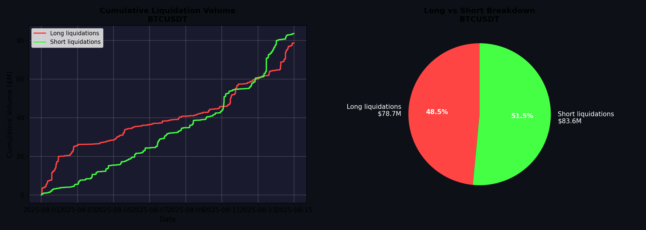
Key observations:
- Nearly balanced over two weeks—neither longs nor shorts dominated overall
- Daily variation: Individual days showed strong imbalances, but they averaged out
- Size distribution: Both sides had similar total volumes but different event distributions
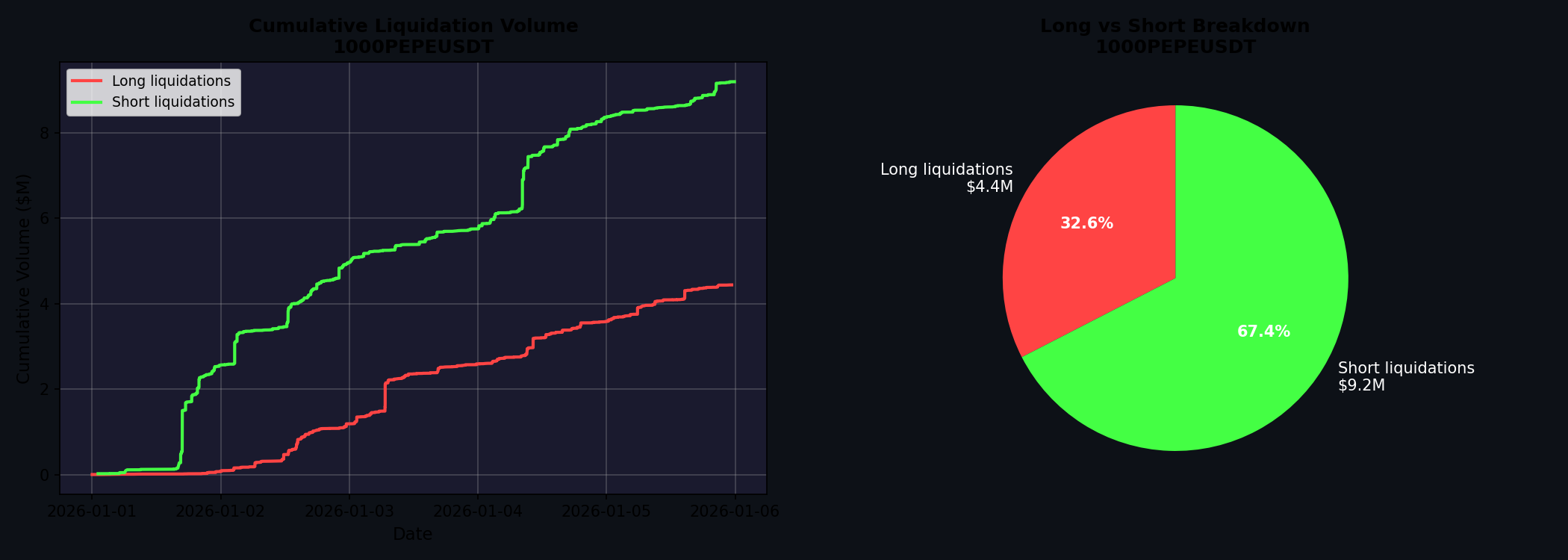
Case Study: 1000PEPEUSDT During 80% Pump
To see how liquidations behave during a strong directional move, let's analyze 1000PEPEUSDT from January 1-5, 2026—a period when the coin rose approximately 80%.
# Load PEPE liquidation data during pump
pepe_df = chd.get_liquidations(
    symbol="1000PEPEUSDT",
    exchange="binance_futures",
    start_date="2026-01-01",
    end_date="2026-01-05"
)
PEPE Liquidation Overview
| Metric | Value |
|---|---|
| Total liquidations | 4,589 |
| Total volume | $13.6M |
| Long liquidations (longs rekt) | $4.4M (32.6%) |
| Short liquidations (shorts rekt) | $9.2M (67.4%) |
During the pump, shorts were liquidated over 2x more than longs. Short sellers betting against the rally got squeezed hard.
Top PEPE Short Liquidation Windows
| Time | Volume | Count | Avg Price |
|---|---|---|---|
| 2026-01-04 08:15 | $669,088 | 37 | $0.0122 |
| 2026-01-01 16:45 | $614,361 | 13 | $0.0098 |
| 2026-01-02 02:35 | $504,086 | 2 | $0.0100 |
| 2026-01-01 16:50 | $342,821 | 6 | $0.0099 |
| 2026-01-02 12:30 | $259,452 | 41 | $0.0105 |
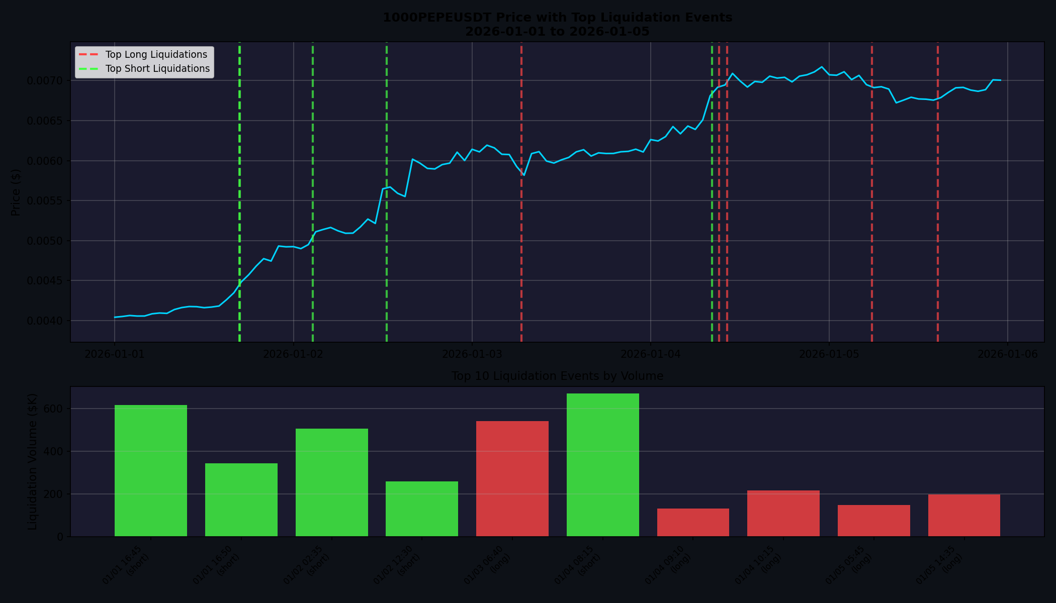
The chart shows the cascade of liquidation events as price rallied—short liquidations (green) dominate as bears got crushed.
PEPE Price Impact
The price impact during the PEPE pump tells a different story:
Long Liquidations:
| Metric | Mean | Median | Min | Max |
|---|---|---|---|---|
| During | -0.45% | -0.13% | -2.03% | +0.41% |
| 1 hour after | +1.11% | +1.21% | -2.57% | +8.37% |
Short Liquidations:
| Metric | Mean | Median | Min | Max |
|---|---|---|---|---|
| During | +0.86% | +0.35% | -0.92% | +5.74% |
| 1 hour after | +2.36% | +2.51% | -0.89% | +6.21% |
Short liquidation events during the pump saw price continue rising +2.36% on average over the next hour—the momentum had legs beyond just the squeeze. The +5.74% move during one short liquidation window shows the violence of a short squeeze in a low-cap altcoin.
Complete Example Code
Here's a complete script for analyzing liquidation data:
import cryptohftdata as chd
import pandas as pd
import numpy as np

# Configure API
chd.configure_client(api_key="your-api-key-here")


def load_and_preprocess(symbol, exchange, start_date, end_date):
    """Load and preprocess liquidation data."""
    liqs_df = chd.get_liquidations(
        symbol=symbol, exchange=exchange,
        start_date=start_date, end_date=end_date
    )

    liqs_df["datetime"] = pd.to_datetime(liqs_df["event_time"], unit="ms")
    liqs_df["price"] = pd.to_numeric(liqs_df["average_price"], errors="coerce")
    liqs_df["quantity"] = pd.to_numeric(liqs_df["filled_quantity"], errors="coerce")
    liqs_df["volume_usd"] = liqs_df["quantity"] * liqs_df["price"]
    liqs_df["liq_type"] = liqs_df["side"].apply(
        lambda x: "long" if x == "SELL" else "short"
    )

    return liqs_df.sort_values("datetime").reset_index(drop=True)


def get_price_timeseries(symbol, exchange, start_date, end_date):
    """Load trade data and create price timeseries."""
    trades_df = chd.get_trades(
        symbol=symbol, exchange=exchange,
        start_date=start_date, end_date=end_date
    )

    trades_df["datetime"] = pd.to_datetime(trades_df["event_time"], unit="ms")
    trades_df["price"] = pd.to_numeric(trades_df["price"], errors="coerce")
    trades_df = trades_df[trades_df["price"] > 0]

    price_df = trades_df.set_index("datetime").resample("1min").agg({
        "price": ["first", "max", "min", "last"]
    }).dropna()
    price_df.columns = ["open", "high", "low", "close"]

    return price_df.reset_index()


def aggregate_by_window(liqs_df, window="5min"):
    """Aggregate liquidations into time windows."""
    df = liqs_df.copy().set_index("datetime")

    agg = df.resample(window).agg({
        "volume_usd": "sum",
        "quantity": "sum",
        "price": "mean",
        "side": "count"
    }).rename(columns={"side": "count", "price": "avg_price"})

    long_agg = df[df["liq_type"] == "long"].resample(window)["volume_usd"].sum()
    short_agg = df[df["liq_type"] == "short"].resample(window)["volume_usd"].sum()

    agg["long_volume"] = long_agg.reindex(agg.index, fill_value=0)
    agg["short_volume"] = short_agg.reindex(agg.index, fill_value=0)

    return agg.reset_index()


def find_top_windows(agg_df, n=10):
    """Find top N windows for long and short liquidations."""
    top_long = agg_df.nlargest(n, "long_volume").copy()
    top_long["type"] = "long"
    top_long["volume"] = top_long["long_volume"]

    top_short = agg_df.nlargest(n, "short_volume").copy()
    top_short["type"] = "short"
    top_short["volume"] = top_short["short_volume"]

    return top_long, top_short


def calculate_price_impact(events_df, price_df, window_minutes=5):
    """Calculate price movement during and after each event."""
    results = []

    for _, event in events_df.iterrows():
        event_time = event["datetime"]
        event_end = event_time + pd.Timedelta(minutes=window_minutes)

        pre = price_df[price_df["datetime"] <= event_time]
        if len(pre) == 0:
            continue
        price_start = pre.iloc[-1]["close"]

        post = price_df[price_df["datetime"] >= event_end]
        if len(post) == 0:
            continue
        price_end = post.iloc[0]["close"]

        result = {
            "datetime": event_time,
            "type": event["type"],
            "volume": event["volume"],
            "change_during": (price_end - price_start) / price_start * 100,
        }

        # Price changes after the event
        for minutes, label in [(5, "5min"), (15, "15min"), (60, "1hr")]:
            after = price_df[price_df["datetime"] >= event_end + pd.Timedelta(minutes=minutes)]
            if len(after) > 0:
                result[f"change_{label}_after"] = (after.iloc[0]["close"] - price_end) / price_end * 100

        results.append(result)

    return pd.DataFrame(results)


def print_summary(liqs_df, symbol):
    """Print analysis summary."""
    total_vol = liqs_df["volume_usd"].sum()
    long_vol = liqs_df[liqs_df["liq_type"] == "long"]["volume_usd"].sum()
    short_vol = liqs_df[liqs_df["liq_type"] == "short"]["volume_usd"].sum()

    print(f"\n{'='*60}")
    print(f"LIQUIDATION ANALYSIS: {symbol}")
    print(f"{'='*60}")
    print(f"Total liquidations: {len(liqs_df):,}")
    print(f"Total volume: ${total_vol:,.0f}")
    print(f"Long liquidations: ${long_vol:,.0f} ({long_vol/total_vol*100:.1f}%)")
    print(f"Short liquidations: ${short_vol:,.0f} ({short_vol/total_vol*100:.1f}%)")


# Run analysis
if __name__ == "__main__":
    # Load BTCUSDT data
    btc_liqs = load_and_preprocess("BTCUSDT", "binance_futures", "2025-08-01", "2025-08-14")
    btc_price = get_price_timeseries("BTCUSDT", "binance_futures", "2025-08-01", "2025-08-14")

    print_summary(btc_liqs, "BTCUSDT")

    # Find top windows
    agg_df = aggregate_by_window(btc_liqs, window="5min")
    top_long, top_short = find_top_windows(agg_df, n=10)

    print("\nTop 10 Long Liquidation Windows:")
    print(top_long[["datetime", "long_volume", "count", "avg_price"]])

    print("\nTop 10 Short Liquidation Windows:")
    print(top_short[["datetime", "short_volume", "count", "avg_price"]])

    # Calculate price impact
    all_top = pd.concat([top_long, top_short])
    impact_df = calculate_price_impact(all_top, btc_price)

    print("\nPrice Impact Summary:")
    for liq_type in ["long", "short"]:
        type_df = impact_df[impact_df["type"] == liq_type]
        print(f"\n{liq_type.title()} liquidations:")
        for col in ["change_during", "change_5min_after", "change_15min_after", "change_1hr_after"]:
            if col in type_df.columns:
                vals = type_df[col].dropna()
                print(f"  {col}: mean={vals.mean():.2f}%, median={vals.median():.2f}%")
Practical Applications
1. Identifying Major Market Events
The top liquidation windows reveal the most significant forced position closures. These often coincide with:
- News events (economic releases, project announcements)
- Technical breakouts (support/resistance breaks)
- Cascade effects (one liquidation triggering another)
2. Sentiment Analysis
The long/short liquidation ratio provides a sentiment signal:
- High long liquidations = overleveraged bulls getting cleared out
- High short liquidations = overleveraged bears getting squeezed
BTCUSDT showed 48.5%/51.5% balance (neutral), while PEPE during the pump showed 32.6%/67.4% (shorts dominating)—classic squeeze territory.
3. Mean Reversion Opportunities
After major long liquidation events, price showed modest recovery (+0.12% average in next 5 minutes). Some traders look for cascade exhaustion as contrarian entry points, though the edge is small and requires careful timing.
Conclusion
Analyzing the top liquidation events directly is more intuitive than statistical threshold approaches. Key takeaways:
- Find the biggest events: Ranking by 5-minute window volume identifies the most significant liquidations
- Long/short ratio reveals bias: 48.5%/51.5% for balanced markets, 32.6%/67.4% during a squeeze
- Price impact varies by context: BTC showed modest -0.21% during long liquidations with small recovery, while PEPE shorts saw +2.36% continuation after squeeze events
- Directional moves amplify effects: The same analysis on PEPE during a pump showed shorts getting liquidated 2x more than longs
Start analyzing liquidation patterns to understand market stress and identify potential opportunities.
Ready to explore liquidation data across different market conditions? Get started with CryptoHFTData and access tick-level liquidation data for all major futures exchanges.