What you'll learn
- How to load orderbook data from CryptoHFTData
- Understanding the structure of L2 orderbook updates
- Basic data exploration and statistics
- Comparing orderbook characteristics across exchanges
Introduction
Orderbook data is the foundation of market microstructure analysis. It shows every change to the limit order book—new orders, cancellations, and fills—giving you visibility into supply and demand that price charts can't provide.
In this tutorial, we'll load a day of BTCUSDT orderbook data from Binance Futures and explore what's inside.
Data: BTCUSDT on Binance Futures, August 1, 2025
Loading Orderbook Data
First, install the SDK and load the data:
pip install cryptohftdata
import cryptohftdata as chd

# Configure with your API key
chd.configure_client(api_key="your_api_key")

# Load orderbook data
orderbook = chd.get_orderbook(
    symbol="BTCUSDT",
    exchange="binance_futures",
    start_date="2025-08-01",
    end_date="2025-08-01",
)

print(f"Loaded {len(orderbook):,} orderbook updates")
# Output: Loaded 154,500,203 orderbook updates
That's 154 million updates for a single day of BTCUSDT. This is true tick-level L2 data.
Understanding the Data Structure
Each row in the orderbook data represents an update to a price level:
print(orderbook.columns.tolist())
Key columns:
| Column | Description |
|---|---|
event_time | When the update occurred (milliseconds) |
side | "bid" or "ask" |
price | The price level being updated |
quantity | New quantity at this level (0 = level removed) |
symbol | Trading pair (BTCUSDT) |
Sample row:
sample = orderbook.iloc[len(orderbook) // 2]
print(f"Time: {sample['event_time']}")
print(f"Side: {sample['side']}")
print(f"Price: ${float(sample['price']):,.2f}")
print(f"Quantity: {float(sample['quantity']):.3f} BTC")
Time: 1754055280520
Side: ask
Price: $115,357.10
Quantity: 0.136 BTC
Basic Statistics
Let's explore the update distribution:
import pandas as pd

# Convert types
orderbook["price"] = pd.to_numeric(orderbook["price"])
orderbook["quantity"] = pd.to_numeric(orderbook["quantity"])
orderbook["datetime"] = pd.to_datetime(orderbook["event_time"], unit="ms")

# Side distribution
print(orderbook["side"].value_counts())
Results from our data:
| Side | Updates | Percentage |
|---|---|---|
| Bid | 79,985,153 | 51.8% |
| Ask | 74,515,050 | 48.2% |
Slightly more bid updates than ask updates on this day.
Update Types
active = orderbook[orderbook["quantity"] > 0]
removed = orderbook[orderbook["quantity"] == 0]

print(f"Active levels (qty > 0): {len(active):,} ({len(active)/len(orderbook)*100:.1f}%)")
print(f"Removed levels (qty = 0): {len(removed):,} ({len(removed)/len(orderbook)*100:.1f}%)")
Active levels (qty > 0): 122,594,233 (79.3%)
Removed levels (qty = 0): 31,905,970 (20.7%)
About 80% of updates are new/modified price levels, 20% are removals (cancellations or fills).
Level Size Analysis
Important: This is L2 (Level 2) orderbook data, which shows the aggregate quantity at each price level—not individual orders. When you see a quantity of 1.5 BTC at $115,000, that could be one order for 1.5 BTC or fifteen orders for 0.1 BTC each. L2 data doesn't distinguish between these cases.
quantities = orderbook[orderbook["quantity"] > 0]["quantity"]

print(f"Mean:   {quantities.mean():.4f} BTC")
print(f"Median: {quantities.median():.4f} BTC")
print(f"Max:    {quantities.max():.2f} BTC")
Mean:   1.2352 BTC
Median: 0.1200 BTC
Max:    1013.56 BTC
The median level size is 0.12 BTC (~$14,000), meaning half of all price levels have less than this amount resting. The maximum of 1013 BTC at a single price level represents significant liquidity concentration—likely from institutional market makers or large limit orders.
Visualizing Update Activity
Let's see how orderbook activity varies throughout the day:
import matplotlib.pyplot as plt

# Resample to 1-minute buckets
df = orderbook.set_index("datetime")
updates_per_min = df.resample("1min").size()

# Plot
fig, ax = plt.subplots(figsize=(14, 5))
ax.plot(updates_per_min.index, updates_per_min.values, linewidth=0.5)
ax.set_xlabel("Time (UTC)")
ax.set_ylabel("Updates per minute")
ax.set_title("Orderbook Update Activity - BTCUSDT Binance Futures")
plt.show()
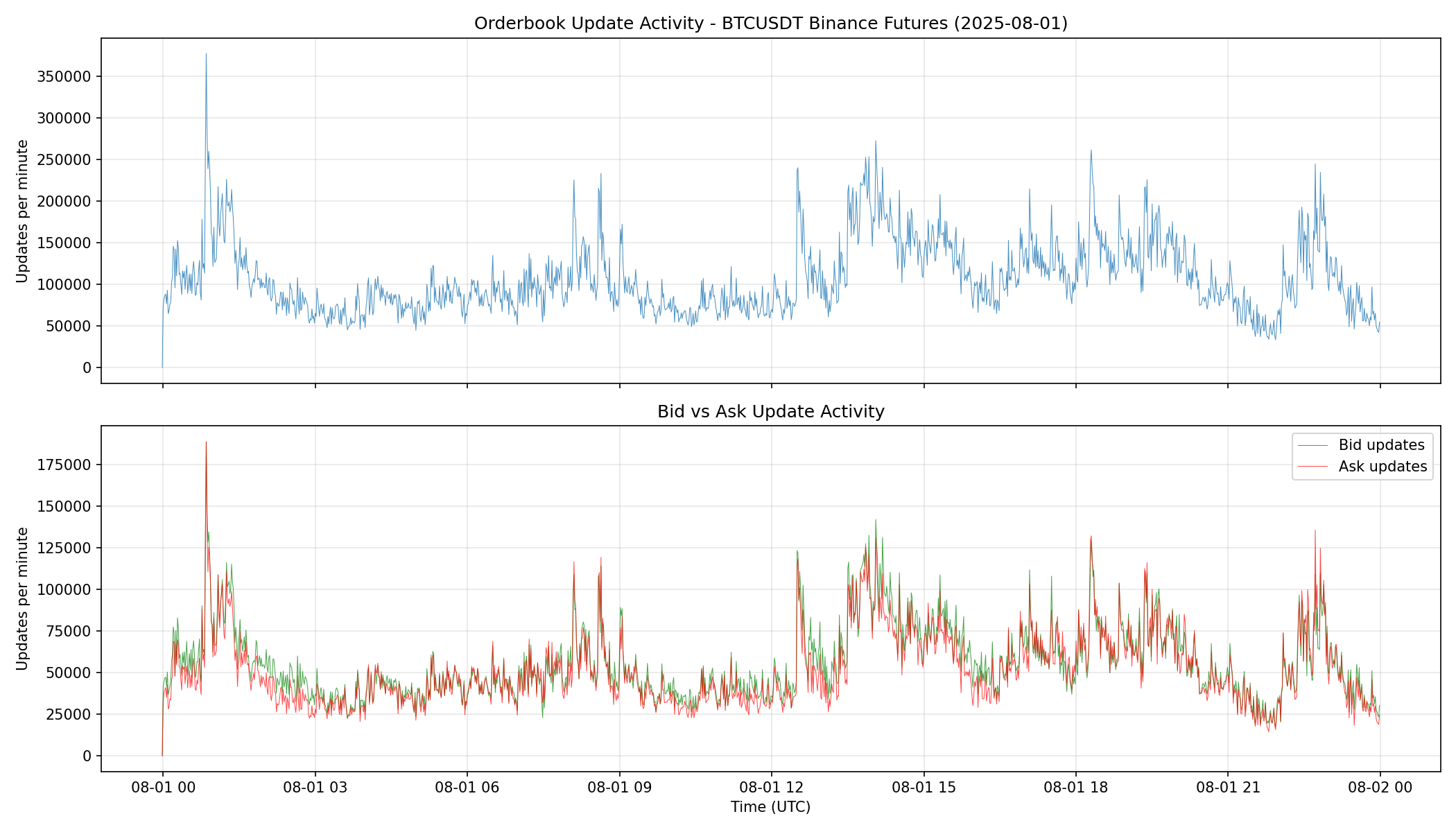
The chart shows:
- Baseline activity: Around 100,000 updates per minute during quiet periods
- Spikes: Activity increases significantly during volatile moments
- Bid vs Ask: Green (bids) and red (asks) tend to move together
Viewing Sample Updates
To see what updates look like at a specific moment:
# Pick a timestamp
sample_time = orderbook["event_time"].iloc[len(orderbook) // 2]
window_ms = 100  # 100ms window

# Get updates in this window
updates = orderbook[
    (orderbook["event_time"] >= sample_time - window_ms) &
    (orderbook["event_time"] <= sample_time + window_ms)
]

# Show bid updates (highest prices)
bids = updates[updates["side"] == "bid"].nlargest(5, "price")
print("BID updates:")
for _, row in bids.iterrows():
    print(f"  ${row['price']:,.2f}  qty: {row['quantity']:.3f}")
BID updates:
  $115,328.90  qty: 27.384
  $115,328.90  qty: 26.573
  $115,328.90  qty: 27.049
  $115,328.70  qty: 0.004
  $115,328.60  qty: 0.001
Note: These are raw updates, not a reconstructed orderbook snapshot. The same price level may appear multiple times as the quantity changes. Full L2 book reconstruction requires processing all updates sequentially to maintain state.
Exchange Comparison: Binance vs Bybit
Different exchanges have different orderbook characteristics. Let's compare Binance Futures and Bybit Perpetuals for BTCUSDT on the same day:
# Load Bybit data
bybit = chd.get_orderbook(
    symbol="BTCUSDT",
    exchange="bybit",
    start_date="2025-08-01",
    end_date="2025-08-01",
)
Head-to-Head Comparison
| Metric | Binance Futures | Bybit Perpetuals |
|---|---|---|
| Total updates | 154,500,203 | 126,590,343 |
| Updates/second | ~1,788 | ~1,465 |
| Bid updates | 79.9M (51.8%) | 62.2M (49.2%) |
| Ask updates | 74.5M (48.2%) | 64.4M (50.8%) |
| Median level size | 0.120 BTC | 0.050 BTC |
| Max level size | 1,013 BTC | 949 BTC |
Key observations:
-
Binance is busier: 22% more updates per day, reflecting higher trading activity and tighter quote updates
-
Bybit has smaller level sizes: Median of 0.05 BTC vs 0.12 BTC on Binance, suggesting more granular liquidity distribution
-
Similar maximum sizes: Both exchanges see ~1000 BTC levels, indicating comparable institutional participation
-
Bid/Ask balance differs: Binance had more bid activity (51.8%), while Bybit was slightly ask-heavy (50.8%)
This kind of cross-exchange analysis is useful for:
- Identifying which venue has better liquidity for your size
- Detecting arbitrage opportunities from update frequency differences
- Understanding market microstructure variations
Key Takeaways
- Volume: A single day of BTCUSDT orderbook data contains 150M+ updates
- L2 vs L3: This is Level 2 data showing aggregate quantities per price level, not individual orders
- Updates vs Snapshots: This is delta data—you see every change as it happens
- Cross-exchange: Different venues have distinct microstructure characteristics
Get Started
pip install cryptohftdata
import cryptohftdata as chd

chd.configure_client(api_key="your_api_key")

orderbook = chd.get_orderbook(
    symbol="BTCUSDT",
    exchange="binance_futures",
    start_date="2025-08-01",
    end_date="2025-08-01",
)
Get your API key at cryptohftdata.com.