What you'll learn
- How to load and process trade data from CryptoHFTData
- Calculating VWAP (Volume Weighted Average Price)
- Measuring buy vs sell pressure from trade flow
- Detecting large "whale" trades
Introduction
Trade data is the raw record of every transaction in a market. Each trade tells you the price, size, and direction—whether a buyer or seller initiated the transaction. This information is essential for understanding market dynamics beyond what candlestick charts can show.
In this tutorial, we'll analyze a full day of BTCUSDT trades from Binance Futures.
Data: BTCUSDT on Binance Futures, August 1, 2025
Loading Trade Data
First, install the SDK and load the data:
pip install cryptohftdata
import cryptohftdata as chd

# Configure with your API key
chd.configure_client(api_key="your_api_key")

# Load trade data
trades = chd.get_trades(
    symbol="BTCUSDT",
    exchange="binance_futures",
    start_date="2025-08-01",
    end_date="2025-08-01",
)

print(f"Loaded {len(trades):,} trades")
# Output: Loaded 4,670,637 trades
That's 4.7 million trades in a single day for BTCUSDT on Binance Futures.
Understanding the Data Structure
Each row represents a single trade execution:
print(trades.columns.tolist())
Key columns:
| Column | Description |
|---|---|
trade_time | When the trade occurred (milliseconds) |
price | Execution price |
quantity | Trade size in base currency (BTC) |
is_buyer_maker | True if buyer was the passive side |
Understanding is_buyer_maker:
is_buyer_maker=True→ Seller was the aggressor (sell pressure)is_buyer_maker=False→ Buyer was the aggressor (buy pressure)
This tells you who initiated the trade, which is crucial for understanding order flow.
Basic Statistics
import pandas as pd

# Convert types
trades["price"] = pd.to_numeric(trades["price"])
trades["quantity"] = pd.to_numeric(trades["quantity"])
trades["volume_usd"] = trades["price"] * trades["quantity"]
trades["side"] = trades["is_buyer_maker"].map({True: "sell", False: "buy"})

# Total volume
total_btc = trades["quantity"].sum()
total_usd = trades["volume_usd"].sum()
print(f"Total volume: {total_btc:,.0f} BTC (${total_usd/1e9:.1f}B)")
Total volume: 221,246 BTC ($25.4B)
$25 billion in volume for a single day—this is why futures markets are the primary venue for institutional trading.
Calculating VWAP
VWAP (Volume Weighted Average Price) is the average price weighted by volume. It's widely used by institutions as a benchmark for execution quality.
VWAP = Σ(price × volume) / Σ(volume)
def calculate_vwap(df, interval="1h"):
    """Calculate VWAP over time intervals."""
    df_indexed = df.set_index(pd.to_datetime(df["trade_time"], unit="ms"))

    # Sum of price × volume
    pv_sum = (df["price"] * df["quantity"]).groupby(
        df_indexed.index.floor(interval)
    ).sum()

    # Sum of volume
    vol_sum = df.set_index(df_indexed.index)["quantity"].resample(interval).sum()

    vwap = pv_sum / vol_sum
    return vwap

vwap_hourly = calculate_vwap(trades, "1h")
Sample VWAP vs Close comparison (hourly):
| Hour | VWAP | Close | Diff (bps) |
|---|---|---|---|
| 00:00 | $115,080.50 | $115,366.90 | +24.9 |
| 01:00 | $115,069.85 | $115,270.20 | +17.4 |
| 02:00 | $115,650.72 | $115,908.80 | +22.3 |
| 03:00 | $115,803.96 | $115,595.70 | -18.0 |
| 04:00 | $115,458.22 | $115,648.30 | +16.5 |
When the close price is above VWAP, buyers were more aggressive in that period. When below, sellers dominated.
Cumulative VWAP
For execution benchmarking, traders track cumulative VWAP throughout the day:
trades["cum_pv"] = (trades["price"] * trades["quantity"]).cumsum()
trades["cum_vol"] = trades["quantity"].cumsum()
trades["cum_vwap"] = trades["cum_pv"] / trades["cum_vol"]
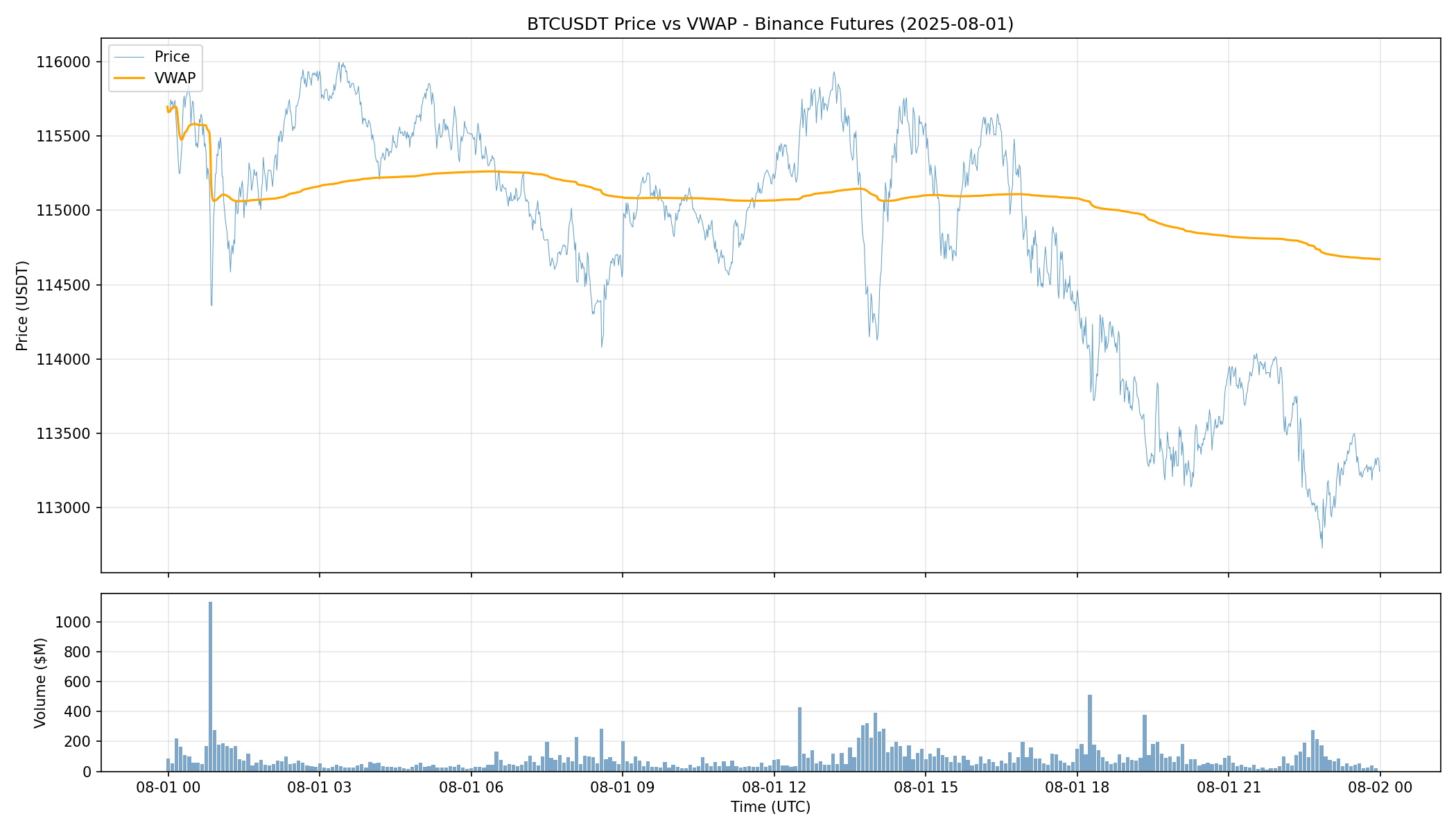
The chart shows price (blue) and cumulative VWAP (orange). VWAP acts as a dynamic support/resistance level—when price is above VWAP, buyers are in control; when below, sellers dominate.
Buy vs Sell Pressure
The is_buyer_maker field reveals the aggressor side of each trade. Aggregating this over time shows where buying or selling pressure is concentrated.
# Calculate per-minute pressure
trades["datetime"] = pd.to_datetime(trades["trade_time"], unit="ms")
df_indexed = trades.set_index("datetime")

buy_vol = df_indexed[df_indexed["side"] == "buy"]["volume_usd"].resample("1min").sum()
sell_vol = df_indexed[df_indexed["side"] == "sell"]["volume_usd"].resample("1min").sum()

# Cumulative delta (buy - sell)
cumulative_delta = (buy_vol.fillna(0) - sell_vol.fillna(0)).cumsum()
Overall pressure for 2025-08-01:
| Metric | Value |
|---|---|
| Buy volume | $12.2B (48.1%) |
| Sell volume | $13.2B (51.9%) |
| Net flow | -$965M |
| Avg buy trade | $5,274 |
| Avg sell trade | $5,587 |
Sellers were slightly more aggressive on this day, with net outflow of nearly $1 billion.
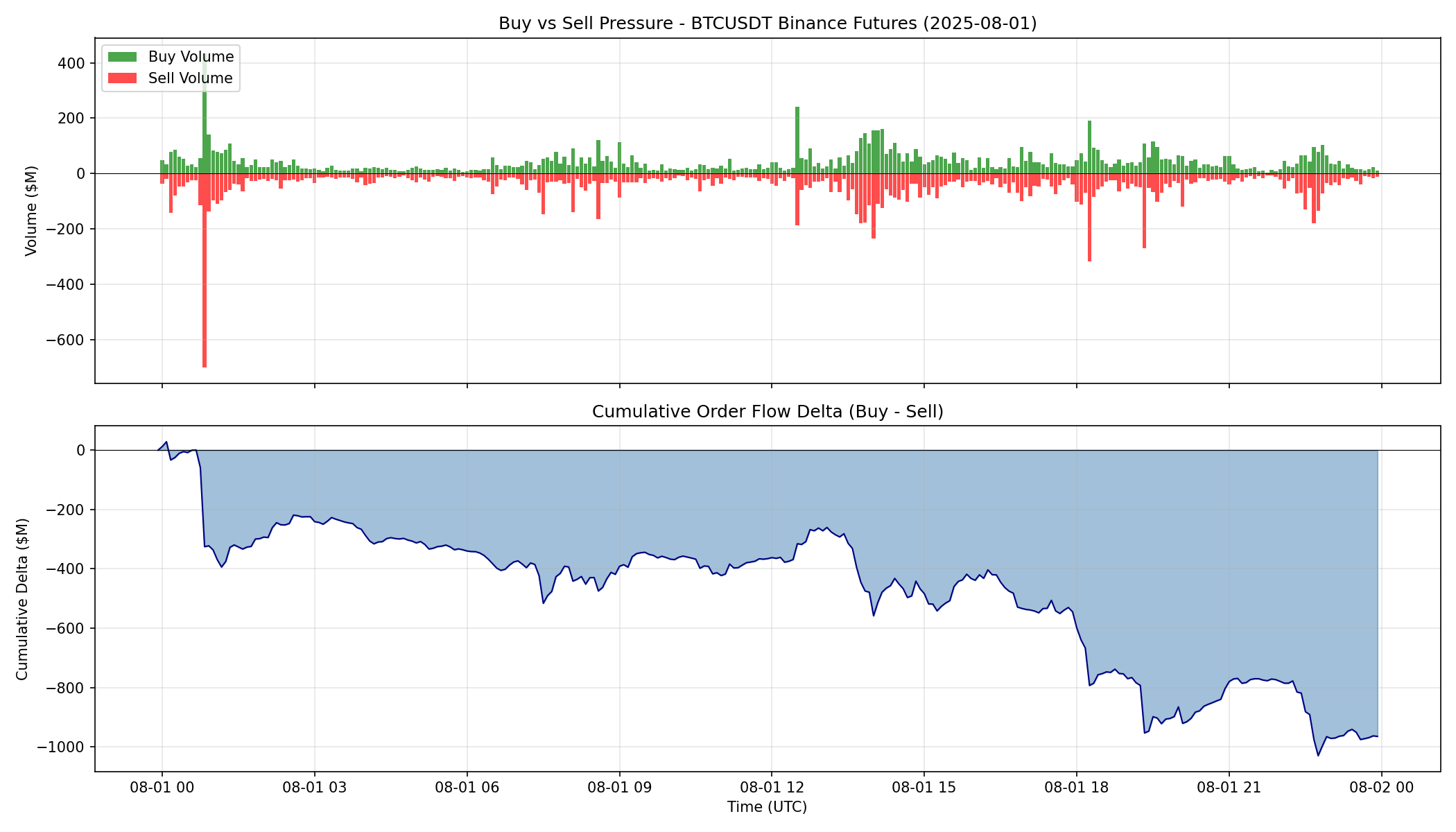
The top panel shows buy (green) vs sell (red) volume over time. The bottom panel shows cumulative delta—the running total of buy volume minus sell volume. A declining cumulative delta indicates persistent sell pressure.
Detecting Whale Trades
Large trades often signal institutional activity or significant market events. However, there's an important nuance: a single large market order may be split into multiple trade events.
When a large market order sweeps through multiple price levels in the order book, each fill at each price level is recorded as a separate trade. These trades share the same event_time timestamp. To accurately measure order sizes, we need to group trades by event_time.
Grouping Trades by Event Time
def group_trades_by_event_time(df):
    """
    Group trades by event_time to reconstruct original market orders.
    A large market order hitting multiple price levels creates multiple
    trade events with the same event_time.
    """
    grouped = df.groupby(["event_time", "side"]).agg({
        "price": "mean",
        "quantity": "sum",
        "volume_usd": "sum",
        "datetime": "first",
    }).reset_index()
    return grouped

# Group 4.7M trades into ~1.2M orders
orders = group_trades_by_event_time(trades)
print(f"Grouped {len(trades):,} trades into {len(orders):,} orders")
Grouped 4,670,637 trades into 1,187,028 orders
Now we can find whale orders using the top 0.1%:
threshold = orders["volume_usd"].quantile(0.999)
print(f"Large order threshold: ${threshold:,.0f}")

whale_orders = orders[orders["volume_usd"] >= threshold]
print(f"Whale orders found: {len(whale_orders):,}")
Large order threshold: $1,636,116
Whale orders found: 1,188
With proper grouping, the threshold for top 0.1% is now $1.64 million—orders of this size represent serious institutional activity.
Top 10 Largest Orders
| Time | Avg Price | Quantity | Value | Side |
|---|---|---|---|---|
| 07:32:56 | $114,800 | 180.52 BTC | $20.7M | Sell |
| 12:46:27 | $115,780 | 89.72 BTC | $10.4M | Buy |
| 16:17:25 | $115,560 | 89.21 BTC | $10.3M | Buy |
| 17:31:01 | $114,835 | 88.69 BTC | $10.2M | Buy |
| 22:34:02 | $113,112 | 88.03 BTC | $10.0M | Sell |
| 12:46:27 | $115,777 | 65.69 BTC | $7.6M | Buy |
| 00:52:23 | $114,330 | 61.71 BTC | $7.1M | Buy |
| 22:43:08 | $112,907 | 62.06 BTC | $7.0M | Sell |
| 15:38:24 | $115,011 | 56.59 BTC | $6.5M | Buy |
| 20:17:12 | $113,184 | 54.26 BTC | $6.1M | Buy |
The largest order of the day was a $20.7 million sell at 07:32 UTC. Without grouping by event_time, this would have appeared as multiple smaller trades—but it was actually a single massive order sweeping through the book.
Whale Order Summary
whale_buys = whale_orders[whale_orders["side"] == "buy"]["volume_usd"].sum()
whale_sells = whale_orders[whale_orders["side"] == "sell"]["volume_usd"].sum()

print(f"Whale buy volume:  ${whale_buys/1e9:.2f}B")
print(f"Whale sell volume: ${whale_sells/1e9:.2f}B")
print(f"Whale net flow:    ${(whale_buys - whale_sells)/1e6:.0f}M")
Whale buy volume:  $1.39B
Whale sell volume: $1.73B
Whale net flow:    -$339M
The top 0.1% of orders (1,188 whale orders) accounted for $3.13 billion in volume—12% of the day's total. Whales were net sellers by $339 million.
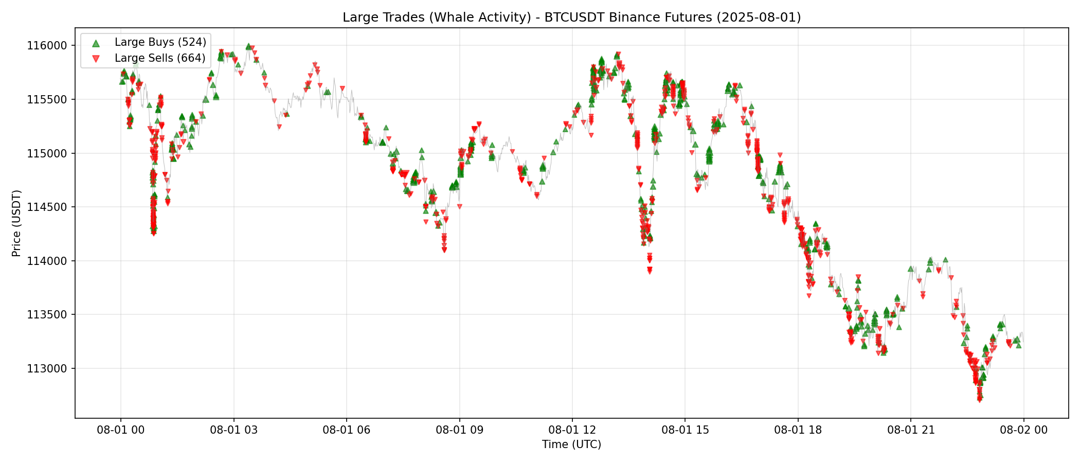
The chart shows price with whale orders (top 0.1%, grouped by event_time) overlaid. Green triangles are large buys, red triangles are large sells. Marker size is proportional to order value. Notice how whale activity clusters around key price levels and during periods of high volatility.
Key Takeaways
- Volume: BTCUSDT on Binance Futures sees 4.7M+ trades and $25B+ in daily volume
- VWAP: A key benchmark that shows whether buyers or sellers are in control
- Order flow: The
is_buyer_makerfield reveals who initiated each trade - Trade grouping: Large orders split across price levels share the same
event_time—group by this to reconstruct true order sizes - Whale detection: Top 0.1% orders (>$1.6M) represent true institutional activity, accounting for 12% of daily volume
Get Started
pip install cryptohftdata
import cryptohftdata as chd

chd.configure_client(api_key="your_api_key")

trades = chd.get_trades(
    symbol="BTCUSDT",
    exchange="binance_futures",
    start_date="2025-08-01",
    end_date="2025-08-01",
)
Get your API key at cryptohftdata.com.